Revisiting Jon Bois' 'What if Barry Bonds Played Without a Bat?'
Introduction
The year is 2004 and Barry Bonds is the most fearsome man in baseball. As evidence of this, Bonds accomplished one of the most impressive feats in sports history - a .609 season on-base pecentage (OBP). To give that number some perspective, consider that the average OBP for a MLB player is around .320 and to have even .400 OBP is all-star level.
In 2017, popular sports storyteller and graphics guru Jon Bois posted What if Barry Bonds had played without a baseball bat? to SB Nation. In it, Bois resimulated all of Bonds’ 2004 plate appearances, replacing all hits, fouls, tips, etc. with either a called strike or a ball. The video is very much worth watching if you haven’t had the pleasure.
After simulating all of this, batless Barry Bonds had an OBP of .608 without a single swing. This seemed unbelievable, even to Bois.
I wanted to revisit Bois’ simulation, but this time repeating Bonds’ 2004 season thousands of times to see if .608 really is a reasonable value, given the constraints of this experiment.
Cleaning the Data
In order to be as close as possible to Jon Bois’ original methodology, I performed the simulation using data provided by Retrosheet.
Retrosheet keeps play-by-play data in it’s own file format called an .evn file, but it’s basically just a textfile.
If you download the entire 2004 season, you will get a zip file with 30 .evn files, one for every team in MLB containing information on the home games for that team.
Retrosheet encodes every plate apperance into a string, ex: BBC*BC>X
How to we convert this weird, text file format into usable, numerical data?
The first step is understanding what individual characters in a plate appearance mean.
Here’s a handy reference for you.
Retrosheet codes:
- C : called strike
- S : swinging strike
- B : ball
- F : foul ball
- L : foul bunt
- M : missed bunt
- Q : swinging strike on pitchout
- R : foul ball on pitchout
- I : intentional ball
- P : Pitchout
- H : Hit by Pitch
- K : strike (not specified)
- X : ball put into play by batter
- T : Foul tip
Obviously this is only step one in a somewhat lengthy process.
The next part is stripping out extraneous characters from the plate appearances.
Here’s the function I wrote to read in .evn files, search for a particular player’s plate appearances, and clean the text strings.
preprocess <- function(filename, player_id = "bondb001", clean = TRUE) {
  require(stringr)
  rawdata <- read.table(filename)
  text <- as.character(rawdata[,1]) # remove header
  data <- data.frame(text = text)

  plays <- as.character(data[grepl("^play*", data$text),])
  events <- unlist(lapply(strsplit(plays[grepl(player_id, plays)], ","), '[', 6))
  outcomes <- unlist(lapply(strsplit(plays[grepl(player_id, plays)], ","), '[', 7))

  if (clean) {

    # Need to remove unnecessary characters
    str_replace(events, "\\*", "") %>%
      str_replace("\\>", "") %>%
      str_replace("\\>", "") %>%
      str_replace("\\.", "") %>%
      str_replace("\\.", "") %>%
      str_replace("\\*", "") %>%
      str_replace("[0-9]", "") %>%
      str_replace("1", "") %>%
      str_replace(">", "") %>%
      str_replace("\\.", "") %>%
      str_replace("\\+", "") -> events
  }

  output <- data.frame(events = events, outcomes = outcomes)
  return(output)

}
Yes, it’s basically a long chain of calls to str_replace, which is true sign of how much this was a process of trial-and-error.
Next step: converting these plate appearances into simulated at-bats according to the rules set by Saint Bois. Again, this means converting fouls, swinging strikes, tips, and balls hit into play into either balls or called strikes. Bois used .191 as the probability that a ball in the strike zone that Bonds didn’t swing at would be a ball, so we will do the same here.
This function is a little long, owing to the fact that I also coded another method of generating a simulated OBP estimate which I’ll discuss in more detail below (that’s what that av = FALSE option is doing in the inputs.
This function will also have to be run on every plate appearance for every simulation run.
convert_pitches <- function(event, p_out = .191, av = FALSE) {

  n <- nchar(event)
  event_av <- event
  for (i in 1:n) {
    if(substring(event, i, i) %in% c("S", "F", "X", "T")) {
      u = runif(1)
      v = 1 - u
      if(u < p_out){
        substring(event, i, i) <- "B"
      } else {
        substring(event, i, i) <- "C"
      }

      if (av) {
        if(v < p_out){
          substring(event_av, i, i) <- "B"
        } else {
          substring(event_av, i, i) <- "C"
        }
      }
    }
  }
  if (av) {
    return(list(event, event_av))
  } else {
    return(event)
  }
}
We’re almost there, now we have to get the final results of each simulated plate appearance. Remember that our simulated Barry Bonds can only walk or strike out looking. In the event that we run out of pitches, we follow the Bois Protocol and simulate some more using .587 as the probability that the pitch will be outside the strike zone.
get_call <- function(event, p_out = .587) {

  ## Returns the call of a plate appearance (either walk or strikeout here)
  ## Inputs: event (string of pitch outcomes) and p_out, the probability a pitch was thrown outside the zone
  ## Output: either "Ball" or "Strikeout"

  count <- list(0, 0)
  n <- nchar(event)
  output <- "none"

  for (i in 1:n) {
    if(substring(event, i, i) == "H") {
      output <- "HBP"
      break
    }
    if(substring(event, i, i) %in% c("B", "I")) {
      count[[1]] <- count[[1]] + 1
    }
    if(substring(event, i, i) == "C") {
      count[[2]] <- count[[2]] + 1
    }
    if(count[[1]] == 4) {
      output <- "Walk"
      break
    }
    if(count[[2]] == 3) {
      output <- "Strikeout"
      break
    }
  }

  # if we run out of pitches, we have to simulate some.
  if (output == "none") {

    while(TRUE) {
      if(rbinom(size = 1, n = 1, p = p_out) == 1) {
        count[[1]] <- count[[1]] + 1
      } else {
        count[[2]] <- count[[2]] + 1
      }

      if(count[[1]] == 4) {
        output <- "Walk"
        break
      }
      if(count[[2]] == 3) {
        output <- "Strikeout"
        break
      }
    }
  }
  return(output)
}
Working with Retrosheet data is a bit laborious since there’s a lot of string manipulation involved. For example, Retrosheet has a multiline encoding for wild pitches which you also need to collapse with if you are going to use this data. My hacky way of handling that ended up looking something like this:
collapse_wild_pitches <- function(events_df) {

  ## WP in retrosheet take up two rows in the .evn -- this function collapses those rows into one
  ## Input: the df output of `preprocess()`
  ## Output: a df with WP pitching outcome rows collapsed into the two right below it

  events_df$events <- as.character(events_df$events)
  events_df$outcomes <- as.character(events_df$outcomes)

  WP <- grep("WP", events_df$outcomes)
  for (row in WP) {
    events_df[row+1, "events"] <- paste(c(as.character(events_df[row,"events"]),
                                          as.character(events_df[row+1,"events"])),
                                        collapse = "")
  }
  events_df <- events_df[-WP,]
  return(events_df)
}
There’s a ton of other little data cleaning bits that I didn’t cover here. However, if you want to drink from the cup of champions, there’s always going to be some sweat involved. And as always, my disclaimer is that I’m not the most talented R programmer, so some of my code may not be the most efficient.
Simulation Methods
I explored two techniques to simulate 2004 batless Bonds’ OBP (that’s a tongue-twister huh):
- Regular Monte Carlo simulation
- Monte Carlo Simulation with antithetic variables
For the Monte Carlo, I wanted to use the exact methodology that Bois used in his video.
We will be generating uniform(0,1) random numbers to simulate pitches. Using the following facts…
- 19.1% of pitches Bonds swung at were outside the zone (a.k.a. they would be called balls in our experiment)
- 58.7% of all pitches thrown to Bonds were outside the zone
…we will be able to covert all of Bonds 2004 swings into called strikes and balls, as well as finish any incomplete PAs in our simulation.
We will also see how the method of antithetic variables affects the variance of our estimates.
This will also involve generating uniform(0,1) random numbers $U_i$, but we will also define and utilize $V_i = 1 - U_i$.
The basic idea behind antithetic variables is that since $U_i$ and $V_i$ are perfectly negatively correlated with one another, the variance of an estimator which is an weighted sum of $U_i$ and $V_i$ should be lower than an estimator based only on either $U_i$ or $V_i$ due to the negative covariance term.
In other words, since $\text{cor}(U_i, V_i) = -1$, we should get an estimate of Bonds’ batless OBP with a smaller variance than the Monte Carlo estimator.
Results
Our Monte Carlo simulations gives us the following distributions with a line at Bois’ original figure of .609 (1000 runs for each method):
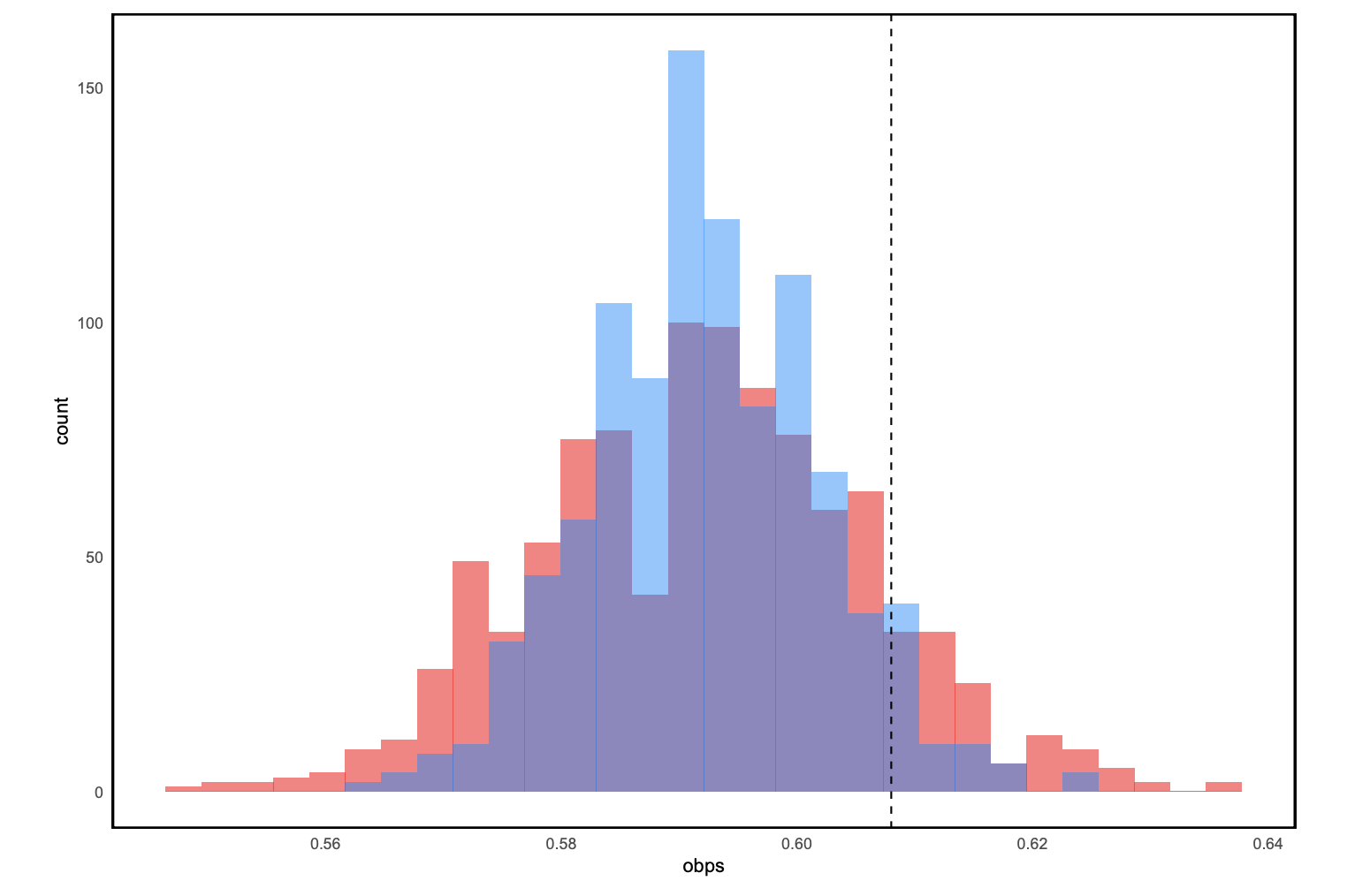
The red histogram are the simulated OBP estimates using regular Monte Carlo simulation. The blue histogram are the simulated OBP estimates using the Monte Carlo with antithetic variables. The method of antithetic variables estimator has a lower variance than the regular Monte Carlo estimator, but that’s about the only part where the simulation methods results differ. Both give an average of around .590… how good is that OBP? Let’s check it with the top single season OBPs in MLB history.
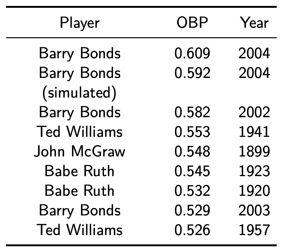
Turns out it’s pretty good. In fact, it’s so good that if we exclude Barry Bonds’ actual 2004 season, this would be the highest OBP of all time.
Conclusion
As with Jon Bois’ original piece, this simulation has no practical sabermetric use. However:
- This simulation showed that Bois’ result was a little on the optimisitic side, but Bonds without a bat according to our simulation rules is still a god-tier player
- We should put Bonds in the HOF. No questions about it.