"The cold queen of England is looking in the glass;
The shadow of the Valois is yawning at the Mass;
From the evening isles fantastical rings faint the Spanish gun,
And the Lord upon the Golden Horn is laughing in the sun."

What did you say you little punk? Fight me IRLS

I took a long hiatus from working on this blog, and will likely continue to have spotty attendance due to a slate of personal events this year, but I have finally completed something I’ve been wanting to do for a long time: calculating coefficients of a logistic regression model “by hand” (e.g. not using glm).

Like many things I write about, there is little practical use for being able to do this. This quality however, apparently makes it a very attractive job interview question. This particular video uses gradient descent like a true machine learning PyChad, but I thought it might be nice to offer an alternative solution using IRLS and R.

ELI5 IRLS PLS

There are a lot of resourced out there which describe iteratively reweighted least squares to varying degrees and varying levels of comprehensibility. Since graduate school, I have tried several times to get an intuitive appreciation for IRLS, but I would immediately run into too more math than I was willing to digest, get discouraged, and close tf out of that browser tab.

The one resource that I found helpful is John Fox’s book Applied Regression Analysis & Generalized Linear Models, a chapter of which can be found online for free. The whole chapter is worth reading, but we can scroll down to page 405 to get right to the good stuff. I’ll do my best now to go through the intuition of the algorithm and then each of the steps.

First, Weighted Least Squares

If you’ve taken a graduate statistics course, you have probably heard of WLS. As the name implies, we basically assign a weight to each observation, which is useful in situations where we have non-constant variance in response variable. In this case, we would weight the observations by the inverse of their estimate variance, so observations that have small variance have a larger weight than those with a high variance.

Intuitively, I think of this as giving the points that are more precise more weight inthe regression model because we “trust” them more (but this is just a mneumonic to keep the logic straight and not an actual technical explanation of the underlying math).

IRLS as you would guess from the name uses concepts from weighted least squares. Observations get weighted, we throw it into some linear algebra, and we get coefficient estimates from it.

Next, Weighted Least Squares but its iterative

GLMs, like ordinary linear regression, are all about modelling conditional distributions e.g. “If I know that my covariates have these particular values, what would the distribution ofmy response variable look like?”

I won’t review GLM components in detail here, but remember that there’s a linear predictor $X\beta$ (commonly seen as $\eta$ in textbooks) that underlies every GLM. This is the part that includes the information from the indepedent variables and looks basically the same as ordinary linear regression.

Ordinary linear regression of course make the assumption of normality, that is, the conditional distribution is a Gaussian centered at the regression line. GLMs are more flexible, in that the conditional distribution can be any distribution that’s an exponential family (I won’t explain this here, mostly because I’m not the expert to do it justice, but know that this includes Gaussian, Poisson, Binomial, Gamma, and all kinds of other stuff).

The collection of these different means $\mu$ for these conditional exponential family distributions is not linear by itself, so we use a link function (usually denoted by $g()$) to make it linear. All $g(\mu_i) = \eta_i$ from your textbook is saying that we are modeling the mean of the conditional distribution by transforming it, then doing a linear regression with unequal variances aka the perfect case for WLS.

Image source

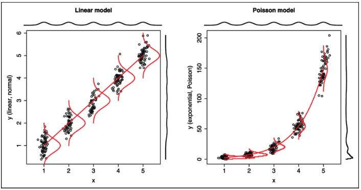
Quick aside: Where do the unequal variances come from? Well, remember that the variances for a lot of these exponential family distributions depend on the mean, so changes depending on $X\beta$, for example, in the binomial distribution, $E[X] = np$ and $Var[X] = np(1-p)$. In the Poisson distibution, both $E[X] = Var[X] = \lambda$. The Gaussian is the special child, since $Var[X] = \sigma^2$, which is constant and doesn’t depend on $\mu$.

This dependence between the variance and mean in the conditional distribution makes WLS tougher though, since we don’t know the values for either! We have indeed reached a circle - the variance depends on the means, and the means depend on the variance via WLS, and the variance depends on the means, etc. etc. However, this circle also automatically gives us the framework for an iterative procedure!

So after all that, we finally get to describing IRLS itself!

"The hidden room in man's house where God sits all the year,
The secret window whence the world looks small and very dear.
He sees as in a mirror on the monstrous twilight sea
The crescent of his cruel ships whose name is mystery;"

1) Define a “working variable”, commonly termed $Z$, which is based on our linear predictor $X_i \beta = \eta_i$

$Z_i = \eta_i + (Y_i - \mu_i)g'(\mu_i)$

I’m using math notation here, but don’t freak out. Just know that this is based on the linear predictor, the residual between the observed data $Y_i$ and the predicted $\mu_i = g^{-1}(\eta_i)$.

The variance $Var[Z_i] = [g’(\mu_i)]^2 \phi Var[\mu_i]$. We’ll ignore the dispersion parameter $\phi$ for now. The important thing to remember is that we have to calculate the variance of $\mu_i$ which for many exponential families is a known formula.

2) We pick initial estimates for $\hat{\mu_i}$ and throw them into the above formulas to get estimates for $Z_i$ and $Var[Z_i]$.

3) We invert the values $Var[Z_i]$ to get the weights which become the entries in an $n \times n$ diagonal matrix.

4) We now calculate WLS regression estimates, for which there is a closed form solution:

$\beta = \left( X^T W X\right)^{-1} X^T W z$

5) We now go back to step 2, but now our estimates for $\mu_i$ are coming from our new $\beta$. We keep repeating this until our coefficient estimates stablize!

TLDR: Iteratively Reweighted Least Squares is just dressed up WLS regression where we are forced to take some extra steps because of the dependence on the mean and variance!

Making Saint Benedict Proud

So let’s try computing a logistic regression model ourselves now. Believe it or not, I think we’re already done with the hard part. Now that we have nailed the intuition, the only thing standing between us and being able to calculate GLM coefficients is wrangling some R syntax and doing a small bit of calculus.

A logistic regression uses a logit link function which looks like

$logit(p) = log\left( \frac{p}{1 - p} \right)$

and has an inverse link function (btw this inverse link function is actually called the logistic function)

$logistic(\eta) = \frac{1}{1 + e^{-\eta}}$

Taking the derivative of the logit function gives us

$logit'(p) = \frac{1}{p(1-p)}$

Finally, the variance function of the Bernoulli distribution is

$Var(p) = p(1-p)$

We can code this real quick in R

logit <- function(x) {
  return(log(x / (1 - x)))
}

logistic <- function(x) {
  return(1 / (1 + exp(-x)))
}

logit_prime <- function(x) {
  return(1 / (x * (1 - x)))
}

V <- function(x) {
  return( x * (1 - x))
}

What else do we need? Ah yeah, we need to define the WLS matrix algebra:

WLS <- function(X, W, z) {
  XtWX <- t(X) %*% W %*% X
  XtWX_inv <- solve(XtWX)
  XtWz <- t(X) %*% W %*% z
  
  return(XtWX_inv %*% XtWz)
}

And I think we also need a function to define the log likelihood function so we have a stopping condition. I skipped over this bit of math, but you can find it pretty easily online.

ll <- function(p, y) {
  ll <- y * log(p) + (1 - y) * log(1 - p)
  return(sum(ll))
}

Now we can throw all these pieces into an IRLS function. Finally!

IRLS <- function(X, y) {
  mu <- rep(.5, length(y))
  delta <- 1
  i <- 1
  
  # initialize log likelihood to 0
  LL <- 0
  
  while (delta > .00001) {
    Z <- logit(mu) + (y - mu) * logit_prime(mu)
    W <- diag(length(Z)) * as.vector((1 / (logit_prime(mu)^2 * V(mu))))
    
    beta <- WLS(X = X, W = W, z = Z)
    eta <- X %*% beta
    mu <- logistic(eta)
    
    LL_old <- LL
    LL <- ll(p = mu, y = y)
    delta <- abs(LL - LL_old)
    
    print(paste0("Iteration: ", i, " LL:", LL, " Beta: ", paste0(beta, collapse = ",")))
    i <- i + 1
  }
}

Time to see if it actually works!

I’ll use the neuralgia dataset that comes with the always useful emmeans package. We’ll be modelling a binary pain variable as a function of treatment, sex, and age, with some interactions. Let’s load this part up real quick and do a logistic regression using good old glm:

library(emmeans)
neuralgia.glm <- glm(Pain ~ Treatment * Sex + Age,
                     family = binomial(link = "logit"),
                     data = neuralgia)
summary(neuralgia.glm)$coe

The coefficients are as follows:

                   Estimate Std. Error    z value    Pr(>|z|)
(Intercept)     -21.0360597 7.02245213 -2.9955433 0.002739564
TreatmentB       -0.9224487 1.63096990 -0.5655829 0.571677355
TreatmentP        2.8268671 1.32063627  2.1405342 0.032311621
SexM              1.4148323 1.32593231  1.0670472 0.285950540
Age               0.2713654 0.09842632  2.7570405 0.005832713
TreatmentB:SexM   0.5110599 1.91824926  0.2664199 0.789915811
TreatmentP:SexM   0.7217635 1.93209017  0.3735662 0.708727107

How does our handwritten IRLS function compare?

X <- model.matrix(neuralgia.glm)
y <- as.numeric(neuralgia$Pain == "Yes")

IRLS(X = X, y = y)

[1] "Iteration: 1 Beta: -10.32487,-0.28145,1.87207,0.93135,0.12793,0.15352,0.05117"
[1] "Iteration: 2 Beta: -16.85133,-0.59977,2.50275,1.29482,0.21442,0.31537,0.37927"
[1] "Iteration: 3 Beta: -20.30882,-0.85531,2.77611,1.40223,0.26136,0.46842,0.65056"
[1] "Iteration: 4 Beta: -21.01231,-0.92004,2.82533,1.41457,0.27104,0.50952,0.7191"
[1] "Iteration: 5 Beta: -21.03603,-0.92245,2.82687,1.41483,0.27137,0.51106,0.72176"

I had my function print out each iteration of IRLS. The final estimates are on the last line, and we can see that they are pretty darn close to the coefficient estimates we get from glm!

I think it would be fun to also replicate the standard errors, but we can probably put a bow in this one for now. Time to pour the mead and crank up the Gregorian chant.

"His turban that is woven of the sunset and the seas.
He shakes the peacock gardens as he rises from his ease,
And he strides among the tree-tops and is taller than the trees,
And his voice through all the garden is a thunder sent to bring.

--"Lepanto" by GK Chesterton