Bigger sample size doesn't always mean more power
Introduction
One of the things taught in intro stats is that the statistical power of a test (the probability of correctly rejecting the null hypothesis, given the null is really false) is influenced by sample size. Even folks with a cursory knowledge of statistics could repeat some version of “the more samples you have, the more power you have”.
This is not true (at least, not all the time).
I recently started working as an applied statistician. A lot of hypothesis tests we conduct is on discrete binomial data e.g. “how many times is something correctly done?” where the parameter of interest is the probability of getting a correct response.
In these situations, power does not increase monotonically with sample size, but forms a sawtooth like pattern which increases on average. In order to demonstrate this, let’s consider a realistic hypothesis testing scenario that a statistician would likely encounter in the wild.
Setup
Say we are testing some product requirement of $p=.90$ when the true value of $p$ is .89 and $\alpha=.01$ for $H_0: p \geq .9$ vs. $H_A: p \leq .9$ We could use some variation of a single proportion hypothesis tests for this, but let’s use a one-sided Clopper-Pearson interval $[1, U]$. We reject when the requirement falls outside of this interval.
Here are two handy functions written in R.
- The first will create a two-sided Clopper-Pearson interval using the Beta distribution, but provided we input an appropriate value of $\alpha$, this function can also give us our 99% one-sided intervals
- The second simulates data using
rbinomand the true value of the parameter $p$ and returns the proportion of the time that the null hypothesized $p_0$ falls outside the Clopper-Pearson interval
clopper_pearson <- function(x, n, alpha) {
	return(
		list(
			lower=qbeta(alpha/2, x, n-x+1),
			upper=qbeta(1-alpha/2, x+1, n-x)
		)
	)
}

power_calc <- function(n, alpha, true_p, req_p, nsims=10000) {
	bounds <- vector(mode = "numeric", length = nsims)
	for (i in 1:nsims) {
		random_sample <- rbinom(1, size=n, prob=true_p)
		cp <- clopper_pearson(x=random_sample, n=n, alpha=alpha*2)
		bounds[i] <- cp$upper
	}
	return(mean(bounds < req_p))
}
Now that $\alpha$ and the hypotheses are fixed, let’s just consider changing the sample size and graph how the power changes.
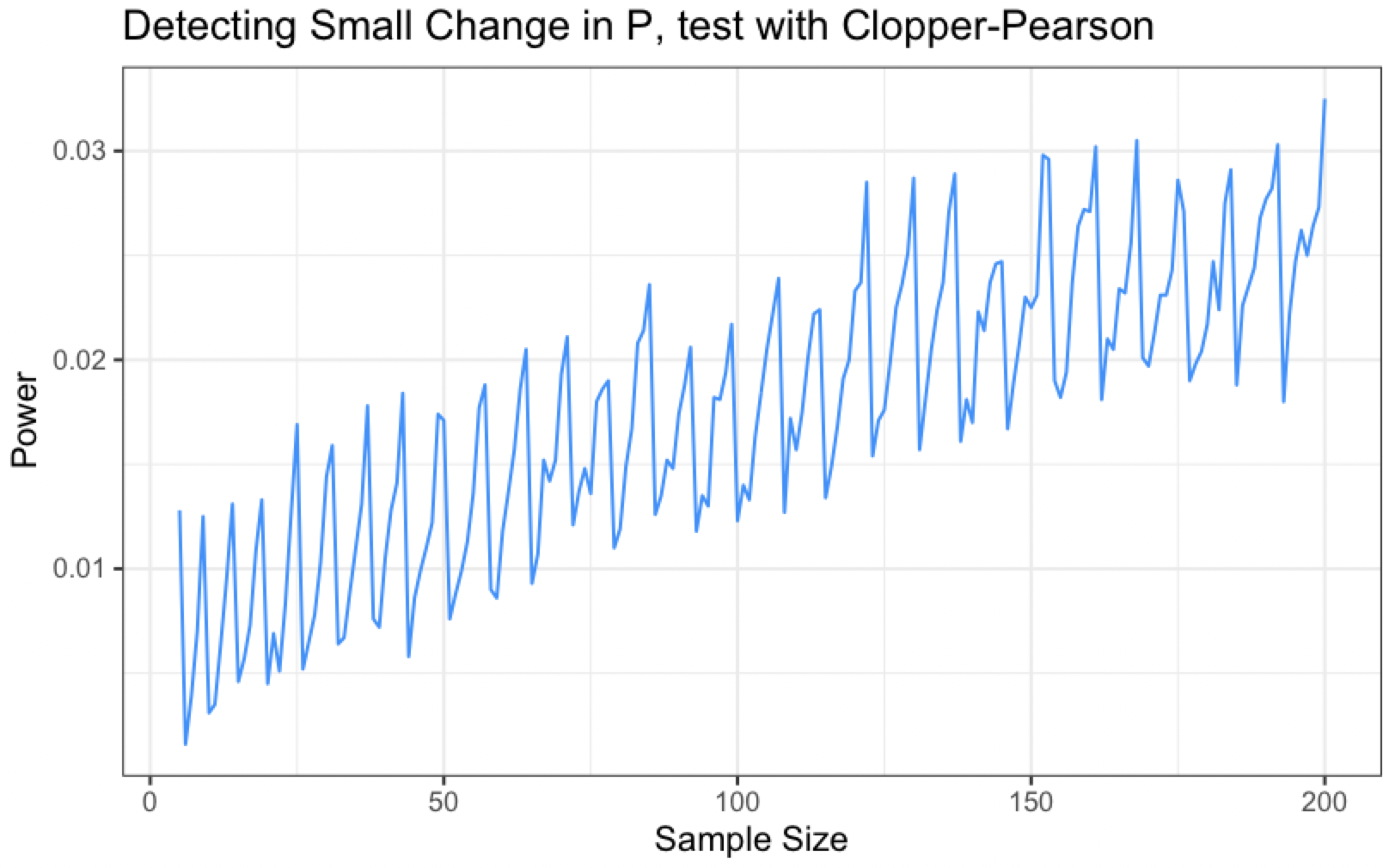
While the overall trend is upwards, it is definitely not monotonic!
This is due to the discrete nature of the data. At any given time, our observed test statistic (the count of correct calls, which Clopper-Pearson intervals are a function of) can only take on so many possible values. This is in contrast to continuous data where the test statistic can take on uncountably infinite values.
In the continuous setting, the rejection region changes with even small changes in the setting of the hypothesis test (consider a standard t-test). However, the rejection region of our $\alpha$-level discrete test does not change quickly enough when the sample size increases are small, and as a result, if we increase sample size by 1 or 2, we are likely to be decreasing the probability that our observed test statistic falls in the unchanging rejection region.
Will randomization smooth this out?
Recall that the reason our power curve is jagged is due to the inability of a discrete test’s rejection region to adjust to small changes in sample size.
The binomial test is a well known hypothesis test for a single proportion in which the test statistic is simple the number of successes $T(x) = \sum x_i$. Let’s consider introducing a randomized component into this test.
If our test statistic falls on the bound of the rejection region, we will reject with some probability $\gamma$ where $\gamma$ is chosen such that the probability of a type I error is exactly $\alpha$. In this way, the rejection region of the discrete test kind of changes even when the hypothesis test setting changes are minute.
First, let’s define a function that can perform a randomized binomial test. The function below will perform such a test for a lower tail hypothesis. Note that $\gamma$ is calculated by taking the difference of $\alpha$ and the probability of falling the rejection region, then dividing that number by the probability of being exactly on the bound of the rejection region.
randomized_binomial_test <- function(x, n, p, alpha) {
	rejection_bound <- qbinom(alpha, size=n, prob=p)
	rejection_region <- rejection_bound - 1
	diff <- alpha - pbinom(rejection_region, size=n, prob=p, lower.tail=TRUE)
	if (diff > 0) {
		gamma <- diff/dbinom(rejection_bound, size=n, prob=p)
	}
	if (x <= rejection_region) {
		return(TRUE)
	} else if (x == rejection_bound) {
		if (runif(1) <= gamma) {
			return(TRUE)
		} else {
			return(FALSE)
		}
	} else {
		return(FALSE)
	}
}
Let’s double check to make sure this function works. Consider a quick example: let’s take a sample of $n=40$ to test $H_0: p \geq .9$ and $H_A: p \leq .9$ at $\alpha=.05$. We can calculate $\gamma$ using the following code.
rejection_region <- qbinom(.05, size=n, prob=prob) -1
rejection_bound <- rejection_region + 1
diff <- alpha - pbinom(rejection_region, size=n, prob=.9, lower.tail=TRUE)
gamma <- diff/dbinom(rejection_bound, size=n, prob=.9)
Running this will return $\gamma=.1405$, meaning that if our test statistic falls on the rejection bound of 33, we should reject the null hypothesis about 14% of the time.
Let’s try it out! Here’s a quick little function that will simulate 10000 randomized binomial tests with a given $x$, $n$, and $p$. Feeding it $x=33, n=40, p=.09$
rbt_sim <- function(x, n, p, alpha, nsim=10000) {
	output <- vector(mode="logical", length=nsim)
	for (i in 1:nsim) {
		output[i] <- randomized_binomial_test(x=x, n=n, p=p, alpha=alpha)
	}
	return(mean(output))
}

rbt_sim(x=33, n=40, p=.9, alpha=.05)
The test rejects ~14% of the time when the observed count is 33, which is precisely the behavior we were looking for.
Let’s wrap our new randomized binomial test function into a simulation helper function and draw some power curves!
rbt_power_calc <- function(n, alpha, true_p, req_p, nsims=10000) {
	outcome <- vector(mode = "logical", length = nsims)
	for (i in 1:nsims) {
		random_sample <- rbinom(1, size=n, prob=true_p)
		outcome[i] <- randomized_binomial_test(x=random_sample, n=n, p=req_p, alpha=alpha)
	}
	return(mean(outcome))
}
Power Curve for Randomized Binomial Test
Consider the above situation again: We are testing a requirement $p=.90$ when the true value of $p$ is .89 and $\alpha=.01$ for $H_0: p \geq .9$ vs. $H_A: p \leq .9$
The power curve for different sample sizes looks like this:
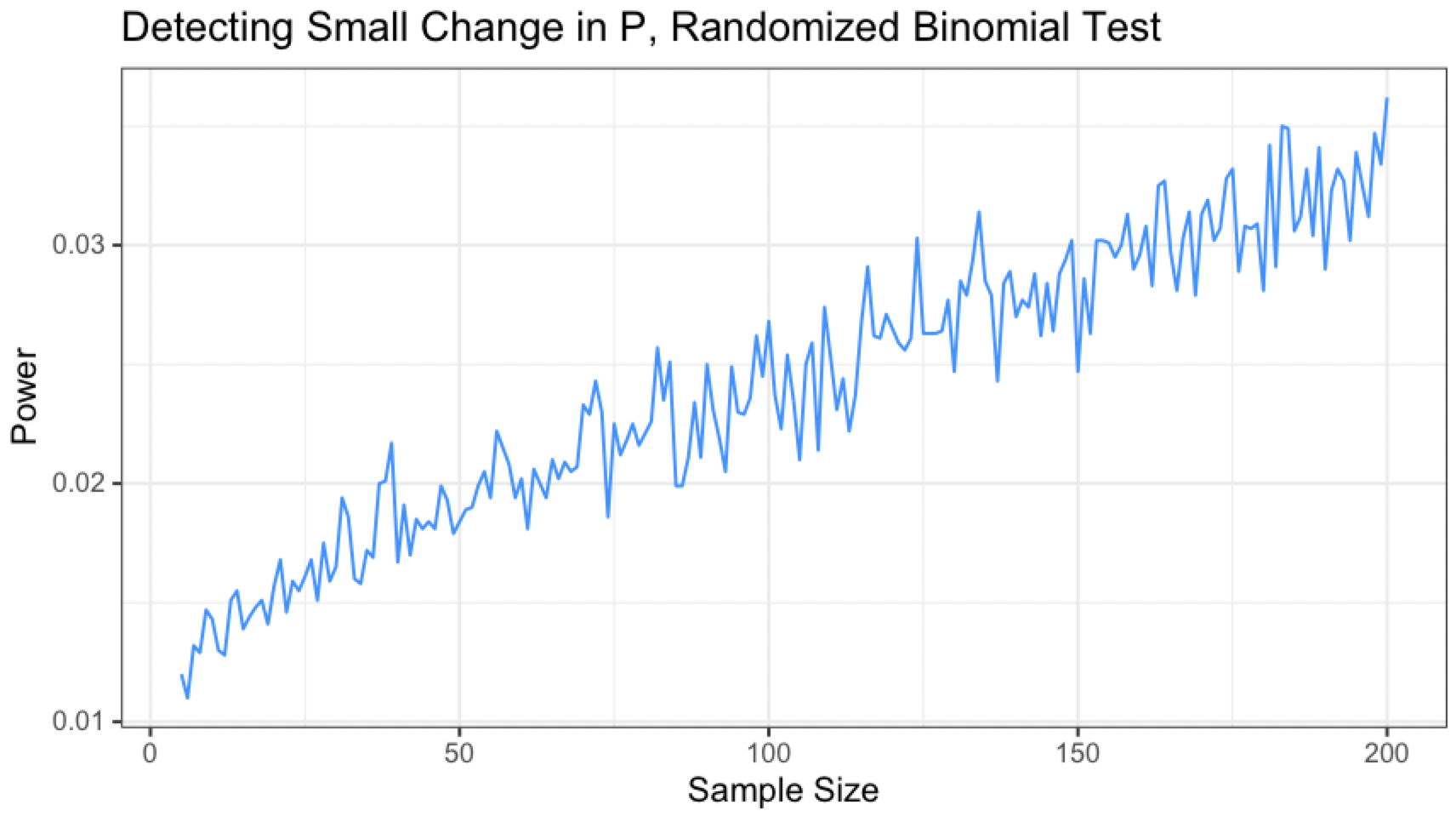
This curve isn’t monotonic either, but interestingly it seems to have lost its periodicity. Although the line’s overall trend is increasing, small dips and hills appear seemingly at random with no repeating pattern.
Comparing the Curves
If we overlay power curve for the Clopper-Pearson interval and the randomized binomial test though, we see that we are making some progress here in flattening the curve (little pandemic reference for you future readers).
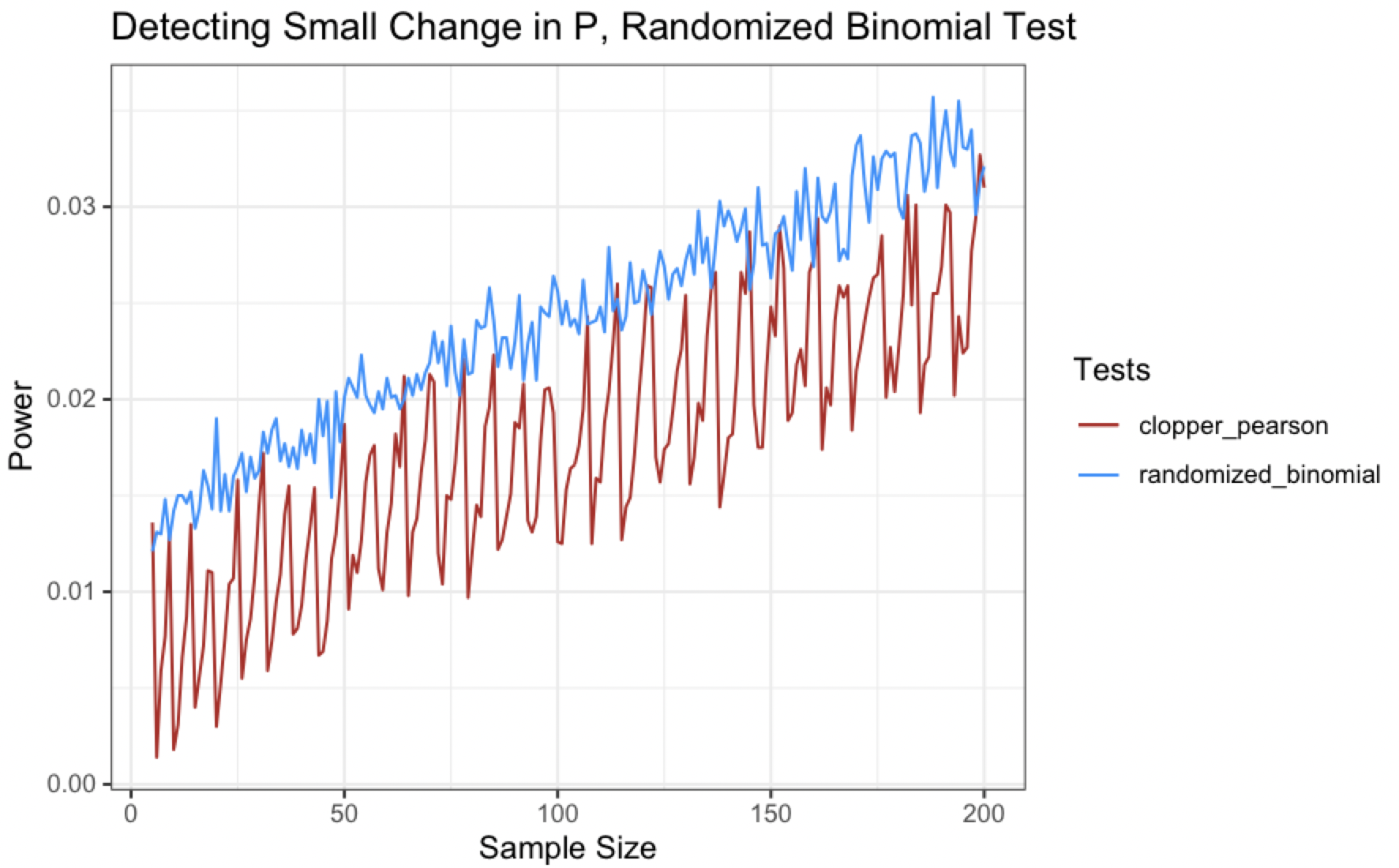
Couple interesting things here:
- The magnitude of the “wiggles” in the power curves is markedly different - the Clopper-Pearson curve has large waves while the randomized binomial test has much less pronounced perturbations
- The power curve for the randomized binomial test actually sits above the Clopper-Pearson curve for most of the sample sizes tested (the power is still pretty low though)
The low overall power for both tests likely stems from the difference between the true probability and required probability being quite small in the above scenario. If we try a different set of hypotheses that are a little more ~boring~ like $H_0:p=.5$ vs. $H_A: p\leq.5$, let’s calculate some power curves for detecting a true probability of $p=.4$ (for a fairly large difference in $p$ of .1).
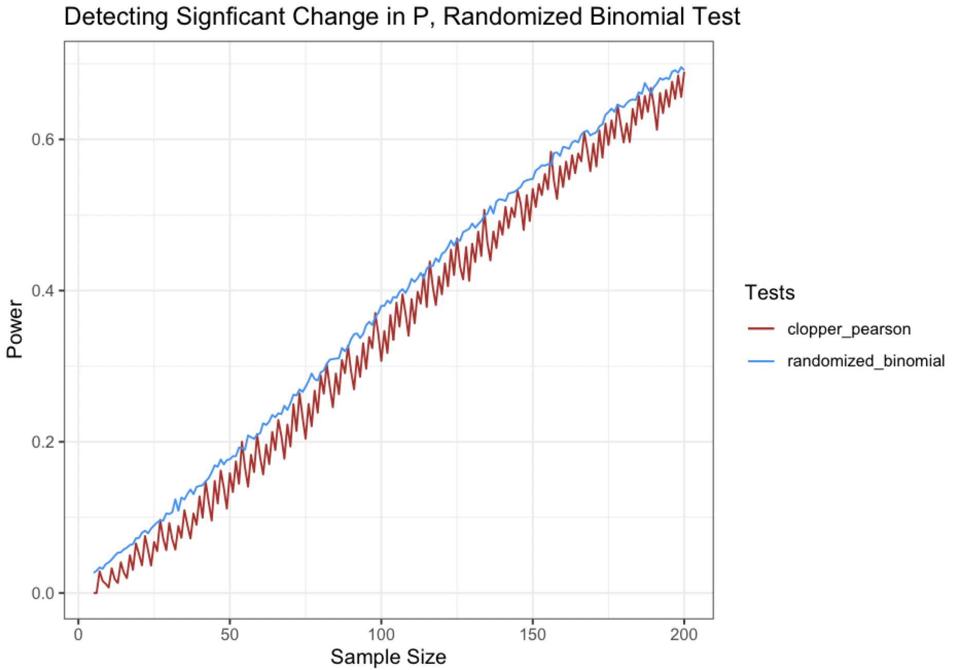
Look at how nice and silky that blue curve is (comparatively speaking, of course)! (^v^)
The bigger the delta between the null hypothesis and the true value of $p$, the smoother we can make our power curves. However, even if we make the differences very large, like .3, it still won’t be perfectly smooth (and in all likelihood, you won’t be seeing many of these testing scenarios in practice). So randomization will not completely smooth out a discrete power curve, but it does show some interesting properties!