(unlimited) power calculations!

Introduction
I had an interview recently for a statistician position which would entail a lot of power and sample size calculations. In school, we learn that statistical power is the probability of a hypothesis test rejecting the null hypothesis if the null hypothesis is, in fact, incorrect. As statisticians, we are able to influence power by
- Changing sample size
- Changing $\alpha$, the probability of type I error
- Changing the alternative hypothesis between two-sided and one-sided hypotheses
- Selecting your sample statistic or designing studies to lower sample variance
And power is also influenced by effect size i.e. it’s easier to detect a big change than a small change!
Now for the actual calculations, we often tasked with finding a particular sample size $n$ to get a desired power while constrained by a certain $\alpha$ and hypothesis. Let’s go over how to think about these calculations and perform some of them for common hypothesis tests.
Binomial test
If you are unfamiliar, the binomial test looks at binary data with an underlying proportion of success with hypothesis $H_0: p = p_0$. The test statistic is simply the number of successes $\sum x_i$ where $x_i$ is your binary data that takes on either a 1 or a 0. This number of success will be distributed according to the binomial distribution, hence the name of the test.
Most introductory statistics classes test proportions using a z-test, but the binomial test has the advantage of not using a normal approximation, hence it is more “exact”. In fact, according to Karlin-Rubin the binomial theorem is the uniformly most powerful test for a single proportion! In some cases, this is advantageous!
We select the rejection region for the test statistic $\sum x_i$ such that $P(\sum x_i \in R \lvert H_0) \leq \alpha$. If our alternative hypothesis is $H_A: p > p_0$, then we will reject the null hypothesis for large values of $\sum x_i$. Our rejection region can be found in R using something like
n <- 100
p0 <- 1/6
alpha <- .05
qbinom(1-alpha, size = n, prob = p0)
In this case, we get 23 so this is the lower bound of our rejection region. If we get $\sum x_i \geq 23$, we can reject the null hypothesis.
However, what if we wanted to calculate the sample size required to detect a difference from the null proportion, say $\delta$? A classical interivew question is to find the sample size required to detect a true proportion of $p_0 + \delta$ with a power of 90%. For the binomial test, we can do this by trying a bunch of sample sizes in increasing order until we get one which satisfies our power requirement. The basic steps will be:
- Generate a list of sample sizes to try
- Calculate the rejection region at each sample size
- Calculate the probability under the true proportion $p_0 + \delta$ of falling into this rejection region
- Return the smallest sample size which reaches the desired power threshold
In R, this would look something like:
n.binomial.test <- function(delta, null.prob = 1/6, req.power = .9, alpha = .05, max.n = 1000) {
	n <- seq(10, max.n, by = 10)
	r <- qbinom(1-alpha, size = n, prob = null.prob)
	power <- pbinom(r, size = n, prob = null.prob + delta, lower.tail = FALSE)
	sample.size <- wihch.max(power > req.power)
	output <- list(
		n <- n[sample.size],
		r <- r[sample.size],
		power <- power[sample.size]
	)
	return(power)
}
1-prop z test
What if we wanted to do this for a one proportion z-test instead of a binomial test? Finding the requisite sample size to get a certain power gets a little more complicated in terms of math, compared to just trying a bunch of sample sizes on a computer. However, it’s still not too difficult!
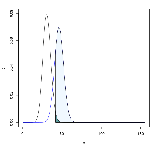
Let’s again consider a null proportion $p_0$ and a true proportion $p = p_0 + \delta$. The general idea is that we want to find the sample size $n$ that sets the $1-\alpha$% quantile of the distribution under the null hypothesis to equal to $1-\text{ power}$% quantile of the distribution under the true value of $p$ (or alternatively, the power% quantile if $\delta < 0$).
Doing a little algebra to figure out a formula for $n$ gives us.
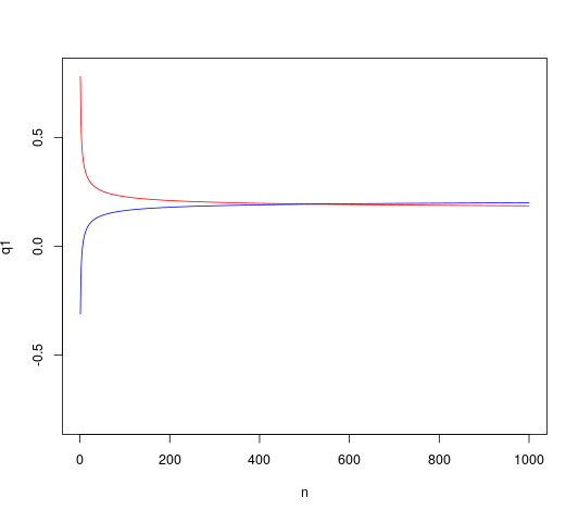
For a very small $\delta$, the sample size required to get the desired power can get infeasibly large. If we are constrained by budgets or practicality, we might have a maximum possible sample size $n_{\text{max}}$. It is possible that the sample sizes available to us do not achieve the desired power without some adjustment in other factors, like $\alpha$. Graphically, this would appear as the quantile functions failing to intersect.
When writing an R function to calculate sample size, we can incorporate this as a check for whether or not we can actually reach power, given our constraints. It might look something like this:
n.calc <- function(p0 = 1/6, alpha = .05, power = .9, nmax = 1000, delta) {
	p <- p0 + delta
	za <- qnorm(1-alpha)
	zb <- qnorm(1-power)
	x <- seq(1, nmax, 1)
	q1 <- p0+za*sqrt(p0*(1-p0)/x)
	q2 <- p+zb*sqrt(p*(1-p)/x)
	if (which.min(abs(q1 - q2)) == nmax) {
		stop("No intersection of quantile functions")
	}
	n <- ((zb*sqrt(p*(1-p)) - za*sqrt(p0*(1-p0)))/(p0-p))^2
	return(round(n))
}
The if block of this function checks for the intersection of the quantile functions. We could have just reported this intersection as our sample size instead of calculating using our formula, but otherwise we did that algebra for nothing so :/
Conclusion
I only explored tests of proportion in this post, but we could easily replicate this general prodedure for a t-test or z-test of a population mean! The key idea here is to think of power calculations in the context of quantiles in different distributions. Once you have that conceptual framework in place, power calculations become a lot friendlier!